
The root locus is one of the concepts used in Stability Analysis.
There are two types of Analysis:
1. Stability Analysis
2. Time Response Analysis
Stability Analysis is of two types:
1. RH criteria
2. Root locus
Time response analysis is of two types:
1. Transient response
2. Steady state response
Table of Contents
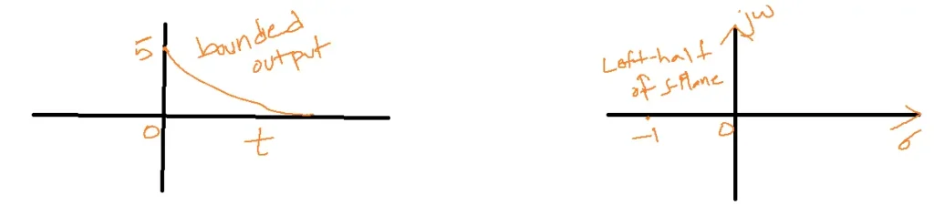
Stability: The system is configured for stability, and if the output is bounded for bounded input, then the output can be controlled.
A signal, either input or output, is said to be limited if its maximum and minimum values are finite.
Examples:
1. 5e-t
s-domain
5/s+1
S+1=0
S=-1
2. 5et
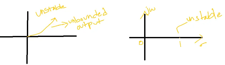
3. 5t- when two poles are located at the origin implies the system is unstable.
4. r(t)=u(t)
The stability of a system depends on the location of poles and does not depend on the location of zeroes.
5. 1/s→ stable system
6. 1/s2→ unstable system
7. e5tsinwt→unstable system
8. e-5tsinwt→stable system
Conditionally stable system:
Consider the transfer function 1/s2+5s+K
In this case, the location of the pole depends on the value of K. Assume that K is varied from 0 to
In some applications, the system will not be stable for all values of K.
A system is deemed limited or conditionally stable if it remains stable only for a subset of K values.
To determine the location of roots the following two techniques are used:
1. R-H criteria
2. Root locus
R-H criteria:
- R-H criteria are applicable for the characteristic equation.
- R-H criteria are also applicable to algebraic equations.
- The characteristic equation is the denominator polynomial of a closed-loop control system.
Example: Determine the stability of a closed loop system whose characteristic equation is given by
S4+4S3-S2+8S+1=0
S4– 1 1 1
S3– 4 8 0
S2– -1 1
S1– 3 0
S0– 1
The order of the characteristic equation is 4.
Roots=4
Two alterations in signs are present. Consequently, two roots are located on the plane’s right half and two on its left half. Therefore the system is unstable.
S4+2S3+10S2+8S+3=0
S4 1 10 3
S3 2 8 0
S2 6 8 0
S1 7 0
S0 3
The system is stable.
Special cases:
Case-1: The first element of the row is zero. When building the RH table, all the elements in the following row will be infinite if 0 appears as the first member in a row. To overcome this problem, the 0 is replaced with a small constant and completes the RH table.
Let E–0 determine the value of elements in the array which are the functions of. The system is stable if there are no further sign changes in the column.
Case-2: A row of all zeroes
An all-zero row indicates the existence of an even polynomial as a factor of a given characteristic equation. If this polynomial the exponents of s are even integers or zero only this is called an auxillary polynomial. The coefficients of auxiliary polynomials will always be the elements of the row directly above the row of the zeroes in the given array.
Root Locus:
The system’s poles or the roots of its characteristic equation determine the stability of the system.
A root locus diagram is used whenever a variable parameter is present in the characteristic equation.
Ex: S2+2S+K=0
The roots of the characteristic equation depend on the value of K.
The root locus technique is used to represent the roots of the C.E graphically when K varies from 0 to infinity. If the system is stable for all the values of K then the system is said to be stable.
The system is considered unstable if the roots are found at the right half of the S-plane as K changes from 0 to infinity. Only for certain values of K are the roots on the left side of the S-plane found in a system that is considered conditionally stable.
Concept of Root locus:
Consider unity negative feedback system
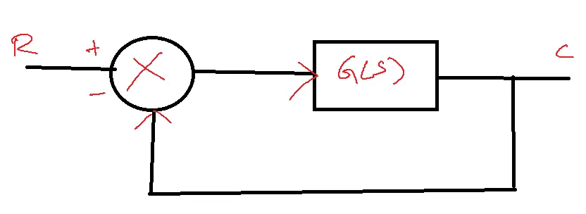
G(S)=K/S+10
CE=1+G(S)=1+K/S+10=0
S+10+K=0
For all the values of K, the roots of characteristic equations or poles are in the left half of the S-plane.
So the system is stable.
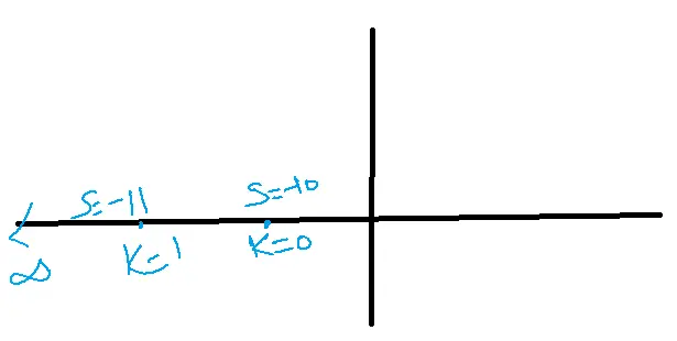
Ex: consider a negative feedback system
G(S)=K/S-10
CE=1+G(S)=1+K/S-10
= S-10+K=0
S=10-K
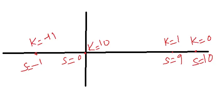
The system is conditionally stable.
K>10 poles are on the left-hand side of the S-plane.
K<10, poles are on the right-hand side of the S-plane.
Rules for sketching the Root locus:
Consider CE 1+G(S)=0
G(S)=-1
|G(S)|=1
G(S)=-1+j0
Magnitude |G(S)|=1
Phase =180 degrees
The roots of the characteristic equation should satisfy the magnitude condition i.e., |G(S)|=1, it is required that the angle equal the odd multiples of 180 degrees.
Rules:
1. The root locus is always symmetrical to the real axis.
2. Number of branches=Number of roots of characteristic equation i.e., Maximum(P or Z) where P and Z are open loop poles and zeroes.
3. Each branch of the root locus starts from the open loop pole i.e., at K=0, and terminates at open loop zero i.e., K=infinity.
Ex: G(S)=K(S+2)/(S+3)
WHEN K=0, 1+G(S)=0
S=-3→ OPEN-LOOP POLE
WHEN K=infinity
S+2=0
S=-2→OPEN-LOOP ZERO
4. If the number of open-loop poles and zeroes to the right of the point is odd, the point on the real axis is in the root locus.
5. The value of K at any point on the root locus can be determined using magnitude criteria. i.e., |g(s)| =1 at S=0.
Problem related to the Root Locus:
Sketch the root locus for a given open loop transfer function G(S)=K(S+10)/S+2. Analyze the stability of the closed-loop system.
Solution: Rule-1:
Number of poles or open loop poles
P=1
S=-2
Number of open loop zeroes
Z=1
S=-10
Rule-2:
Number of branches=Maximum of P or Z=1
1+G(S)=0
When K=0
S=-2 open-loop pole
When K= infinity
S+2+K(S+10)=0
S=-10 open-loop zero.
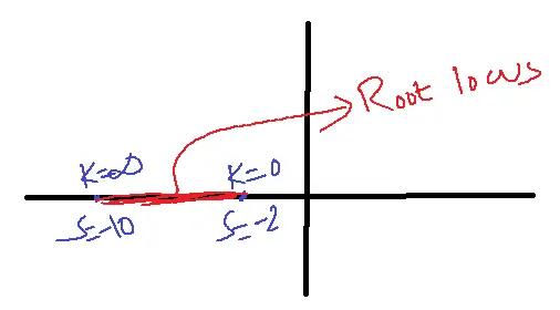
As K varied from 0 to infinity, the roots of the CE are the left half of the S-plane.
Therefore the system is stable.
6. When P≠Z(P>Z) P-Z branches terminates along straight line asymptotes.
7. The angle of asymptotes = (2q+1)1800/P-Z where q=0,1,2,3,….P-Z-1
8. The asymptotes will intersect the real axis at the centroid.
Centroid=sum of real parts of poles-sum of real parts of zeroes/ P-Z.
Note: The above three rules (6,7,8) are applicable only when P≠Z.
9. A breakaway point, also called a breaking point, is necessary if the root locus is between two poles or two zeroes. Solve dk/ds=0 to find the break-away or break-in point.
10. If the open loop transfer function consists of complex poles, an angle of departure is required.
The angle of departure formula:
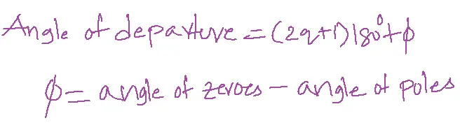
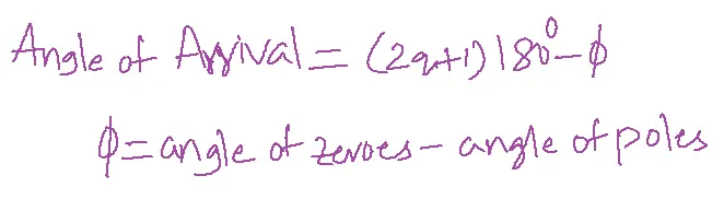
If the open loop transfer function consists of complex zero, an angle of arrival is required.
The angle of arrival formula:
11. The point of intersection on the root locus with the imaginary axis can be determined by using R-H criteria.
Example: The open loop transfer function G(S)=K/S(S+10) sketches the root locus and analyzes the stability.
Sol: P=2, Z=0
Number of branches=Max(P,Z)=2
P-Z=2 branches are terminating along straight-line asymptotes.
When K=0àS=0,S=-10
When K=infinity, no zeroes.
Asymptotic angle= (2q+1)1800/P-Z
q=P-Z
q=(0,1)
q=0→q=900
q=1→q=2700.
Centroid=(0-10)-0/2=-5
CE→1+G(S)=0
1+K/S(S+10)=0
K=-S2-10S
S=-10.
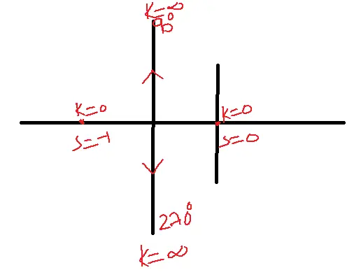
Possessing a breakaway point is necessary since the root locus is situated between two poles.
dk/ds=0
As K varied from 0 to both the roots are located at the left half of the S-plane.
Therefore the system is stable.
Related FAQs
Q1: What is the root locus in control systems, and why is it important for ECE students?
- The root locus is a graphical method used in control systems engineering to analyze how the closed-loop poles of a system change as a specific parameter (usually gain) varies.
- It’s essential for ECE students as it helps assess stability, design compensators, and understand system behavior.
Q2: How do I construct a root locus plot for a given control system?
- Constructing a root locus plot involves following specific rules and steps, such as identifying open-loop poles and zeros, determining the number of branches and their asymptotes, and finding breakaway/break-in points. Software tools like MATLAB can simplify this process.
Q3: What insights into system stability can be derived from a root locus plot?
- A root locus plot reveals whether a system is stable or unstable based on the location of its closed-loop poles.
- The system is considered unstable if its poles are located in the right half of the complex plane.
- The plot also helps determine the stability margin and design controllers for desired performance.
Q4: How does the root locus technique aid in the design of compensators for control systems?
- Root locus provides valuable insights into how compensators (e.g., lead, lag, or lead-lag) can be designed to modify the closed-loop pole locations and achieve desired system response characteristics, such as faster settling time, reduced overshoot, or improved stability margins.
Q5: Which prevalent misunderstandings and difficulties surround root locus analysis in control systems?
- Challenges in root locus analysis include dealing with complex systems, high-order systems, or systems with multiple parameters.
- Misinterpretations of the plot or misunderstandings of the technique’s constraints can occur.
- Proper understanding and practice are crucial for effective utilization.